• February 10, 2025
• 6 min read

Anomaly Detection with Isolation Forest and Qdrant

This beginner tutorial uses the Isolation Forest algorithm for anomaly detection and Qdrant for storage and visualization.

In this specific demo, we will explore a Stronghold ruin and look for ghosts. Our hero will go through all the Shadows and see if he can come across anomalies, aka Wraiths. Take a look at the YouTube demo:

👉 To just run the code - here is the Python notebook

Introduction

This tutorial will guide you through implementing an anomaly detection system using Qdrant, a vector search database, and the Isolation Forest algorithm from Scikit-Learn. By the end of this tutorial, you will:

1. Generate synthetic data containing normal and anomalous samples.
2. Store and retrieve vector embeddings in Qdrant.
3. Train an Isolation Forest model for anomaly detection.
4. Update Qdrant with anomaly labels and visualize results using PCA.
5. Visualize vectors and anomalies in Qdrant.

Prerequisites

1. Install and run Qdrant locally. Here is the documentation.

2. Ensure you have the necessary libraries installed. Run the following command:

pip install qdrant-client scikit-learn numpy matplotlib

Step 1: Import Dependencies

First, import the required libraries:

import numpy as np
import matplotlib.pyplot as plt
from qdrant_client import QdrantClient
from qdrant_client.models import PointStruct, VectorParams, Distance
from sklearn.ensemble import IsolationForest

• numpy: Used for numerical operations and data generation.
• matplotlib.pyplot: Used for visualization.
• qdrant_client: Qdrant's Python client for vector storage and retrieval.
• IsolationForest: The algorithm used for anomaly detection.

Step 2: Generate Synthetic Data

To simulate real-world data, we create 490 normal data points that are randomly distributed around a mean value of 0.5 with some variance. Additionally, we generate 10 anomalous data points that are positioned further away, making them easier to detect.

# Set random seed for reproducibility
np.random.seed(42)

# Generate normal embeddings (centered around 0.5)
normal_data = np.random.normal(loc=0.5, scale=0.1, size=(490, 128))

# Generate anomalies (farther from the normal cluster)
anomalies = np.random.normal(loc=1.5, scale=0.3, size=(10, 128))

# Combine normal and anomalous data
data = np.vstack([normal_data, anomalies])

# Print data shape
print(f"Generated {data.shape[0]} vectors of dimension {data.shape[1]}")

By keeping anomalies at a different mean value (1.5), they are positioned distinctly from the normal points, making them detectable through distance-based methods.

Step 3: Connect to Qdrant and Create a Collection

Qdrant is a vector search engine that allows efficient similarity search. In this specific tutorial, we will only use Qdrant to store vectors and to visualize their distribution. The anomaly detection will be handled by the Isolation Forest algorithm.

In another tutorial, we will use Qdrant's API to detect outliers. For now, Qdrant can be used to store and retrieve vectors at great speeds.

We first connect to a locally running instance and create a collection named Stronghold, specifying a 128-dimensional vector space using cosine distance as the similarity measure.

# Connect to Qdrant (Assuming running locally)
client = QdrantClient("http://localhost:6333")

# Create a collection (if it doesn't exist)
collection_name = "Stronghold"

client.recreate_collection(
    collection_name=collection_name,
    vectors_config=VectorParams(size=128, distance=Distance.COSINE)
)

Step 4: Insert Data into Qdrant

We now insert the generated data points into the Qdrant database. Each data point is assigned an ID and stored with a default label unknown.

# Insert data into Qdrant
points = [
    PointStruct(id=i, vector=vector.tolist(), payload={"label": "unknown"})
    for i, vector in enumerate(data)
]
client.upsert(collection_name=collection_name, points=points)

print(f"Inserted {len(points)} vectors into Qdrant.")

Open up Qdrant Dashboard on http://localhost:6333/dashboard. Your collection should be there, with the appropriate config.

Step 5: Retrieve Stored Vectors

To validate that the data has been successfully stored, we retrieve the stored vectors from Qdrant.

retrieved_points = client.scroll(collection_name=collection_name, limit=500)[0]

# Extract vectors and IDs
retrieved_vectors = np.array([point.vector for point in retrieved_points if point.vector is not None])
retrieved_ids = [point.id for point in retrieved_points]

print(f"Retrieved {len(retrieved_vectors)} vectors from Qdrant.")

Step 6: Train Isolation Forest for Anomaly Detection

We train an Isolation Forest model to detect anomalies in the dataset. Isolation Forest works by isolating anomalies, which typically require fewer splits compared to normal points.

# Train Isolation Forest model
iso_forest = IsolationForest(contamination=0.05, random_state=42)
predictions = iso_forest.fit_predict(data)

# Convert predictions (-1 = anomaly, 1 = normal)
anomaly_labels = ["Wraith" if p == -1 else "Shadows" for p in predictions]

# Count anomalies
print(f"✅ Detected {anomaly_labels.count('Wraith')} anomalies out of {len(data)} vectors.")

Step 7: Update Qdrant with Anomaly Labels

We now update the stored vectors in Qdrant with their anomaly classification.

# Update payloads in Qdrant with anomaly labels and image URLs
for i, point_id in enumerate(retrieved_ids):
    # Define image URL based on label
    image_url = "https://i.ibb.co/Q7z72wq3/shadows.png" if anomaly_labels[i] == "Shadows" else "https://i.ibb.co/NnS6DV5z/wraith.png"

    client.set_payload(
        collection_name="Stronghold",
        points=[point_id],
        payload={
            "anomaly": anomaly_labels[i],
            "image_url": image_url
        }
    )
print("✅ Updated Qdrant with anomaly labels and image URLs.")

Step 8: Discover Anomalies with Qdrant

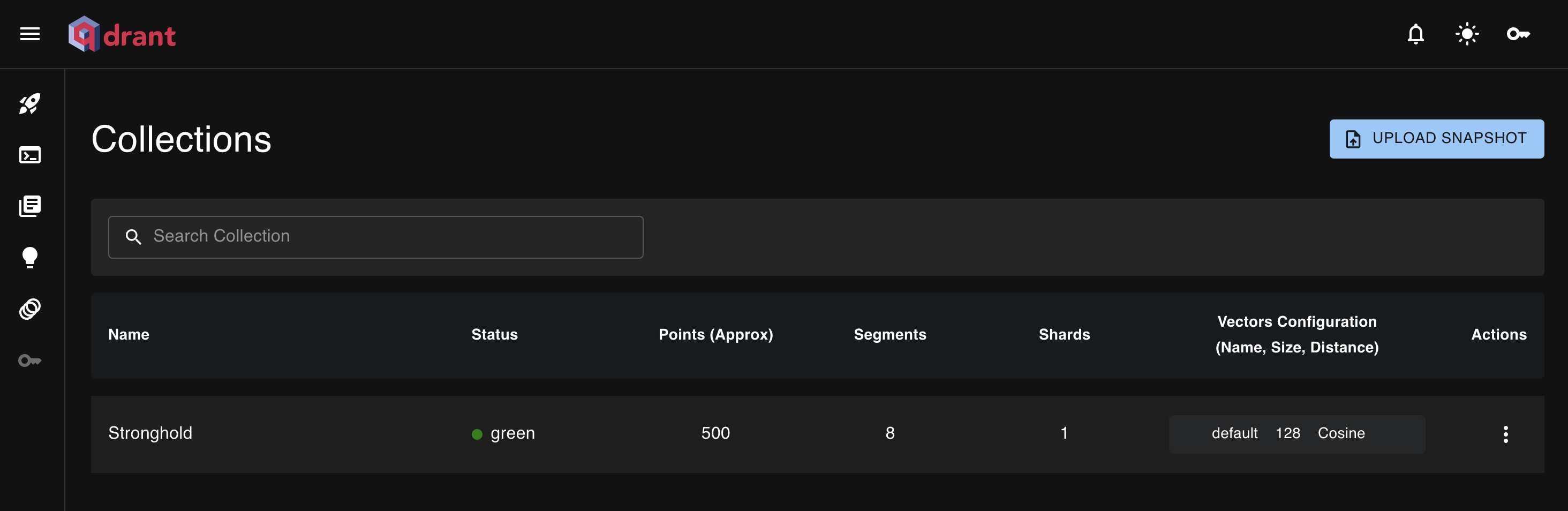
Qdrant provides a web UI where you can inspect the stored vectors and their associated metadata.

1. Open your web browser and go to http://localhost:6333/dashboard.

2. Navigate to the Stronghold collection.

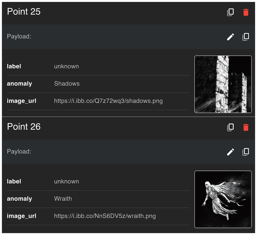
3. Use the search functionality to inspect vectors labeled as anomalies (Wraith).

4. You can filter by payload: anomaly: Wraith.

Step 9: Visualize Anomalies with PCA

To visualize the results, we use Principal Component Analysis (PCA) to reduce the vector dimensions to 2D for plotting.

from sklearn.decomposition import PCA
import matplotlib.pyplot as plt

# Reduce dimensions to 2D using PCA
pca = PCA(n_components=2)
data_2d = pca.fit_transform(data)

# Assign colors based on anomaly labels
colors = ["red" if label == "Wraith" else "blue" for label in anomaly_labels]

# Scatter plot
plt.figure(figsize=(10, 8))
plt.scatter(data_2d[:, 0], data_2d[:, 1], c=colors, alpha=0.7)
plt.xlabel("PCA Component 1")
plt.ylabel("PCA Component 2")
plt.title("Anomaly Detection Visualization")
plt.show()

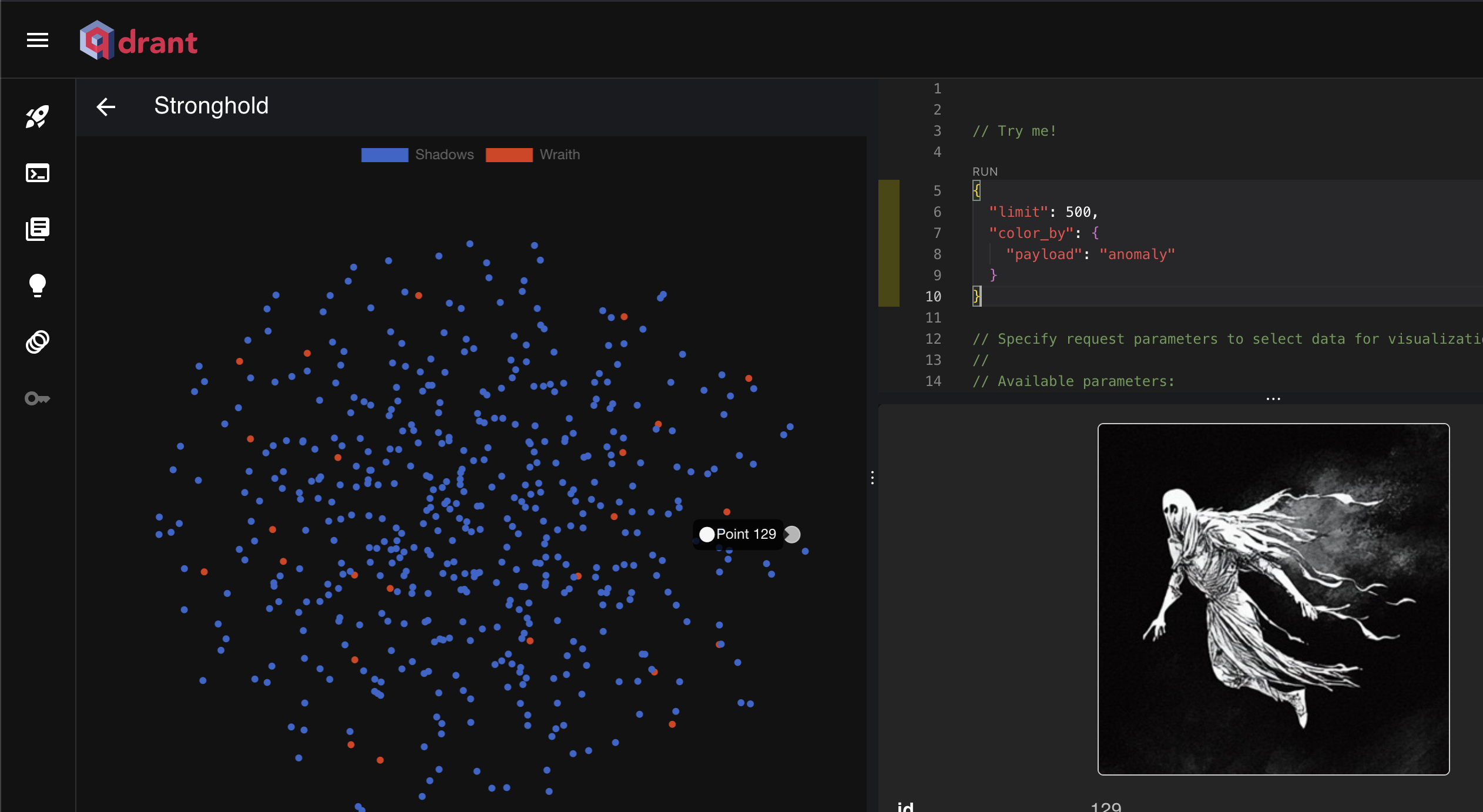
Step 10: Visualize Anomalies with Qdrant

Use the visualization feature of Qdrant to inspect vectors labeled as anomalies (Wraith).

Here is a sample json configuration for to generate the graph:

{
  "limit": 500,
  "color_by": {
    "payload": "anomaly"
  }
}

Explore the associated image URLs and metadata to understand how anomalies are distributed.

You can hover over each point and see the content of the metadata.

👉 To just run the code - here is the Python notebook

Conclusion

This tutorial demonstrated how to:

1. Generate synthetic data.
2. Store and retrieve vectors in Qdrant.
3. Train an Isolation Forest model for anomaly detection.
4. Update Qdrant with anomaly labels.
5. Visualize anomalies using PCA.

With these techniques, you can apply anomaly detection in real-world scenarios like fraud detection, network intrusion detection, and more!